Practical 3: Markov Decision Processes

# # Practical 3: Markov Decision Processes

import numpy as np
import matplotlib.pyplot as plt


# ## Markov Chain

# Define a transition matrix

n_states = 10
idx = np.arange(n_states)
transition_matrix = np.zeros((n_states, n_states))
transition_matrix[idx, (idx - 1) % n_states] = 0.1
transition_matrix[idx, (idx + 1) % n_states] = 0.9
transition_matrix[0, 0] = 0.8
transition_matrix[0, 1] = 0.1
transition_matrix[0, -1] = 0.1
print(f"normalised: {np.all(transition_matrix.sum(axis=1)==1)}")


# Sample and plot episodes

normalised: True

def sample_episodes(n_episodes, length_episodes):
    episodes = np.zeros((n_episodes, length_episodes), dtype=int)
    for idx_episodes in range(n_episodes):
        for idx_time in range(1, length_episodes):
            current_state = episodes[idx_episodes, idx_time - 1]
            probs = transition_matrix[current_state]
            next_state = np.random.choice(n_states, p=probs)
            episodes[idx_episodes, idx_time] = next_state
    return episodes

episodes = sample_episodes(n_episodes=10, length_episodes=100)
fig, ax = plt.subplots(1, 1, figsize=(15, 10))
ax.plot(np.arange(episodes.shape[1]), episodes.T, '-o', alpha=0.3);


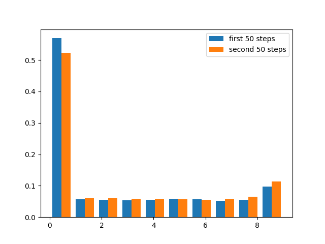
# Plot statistics of state visits

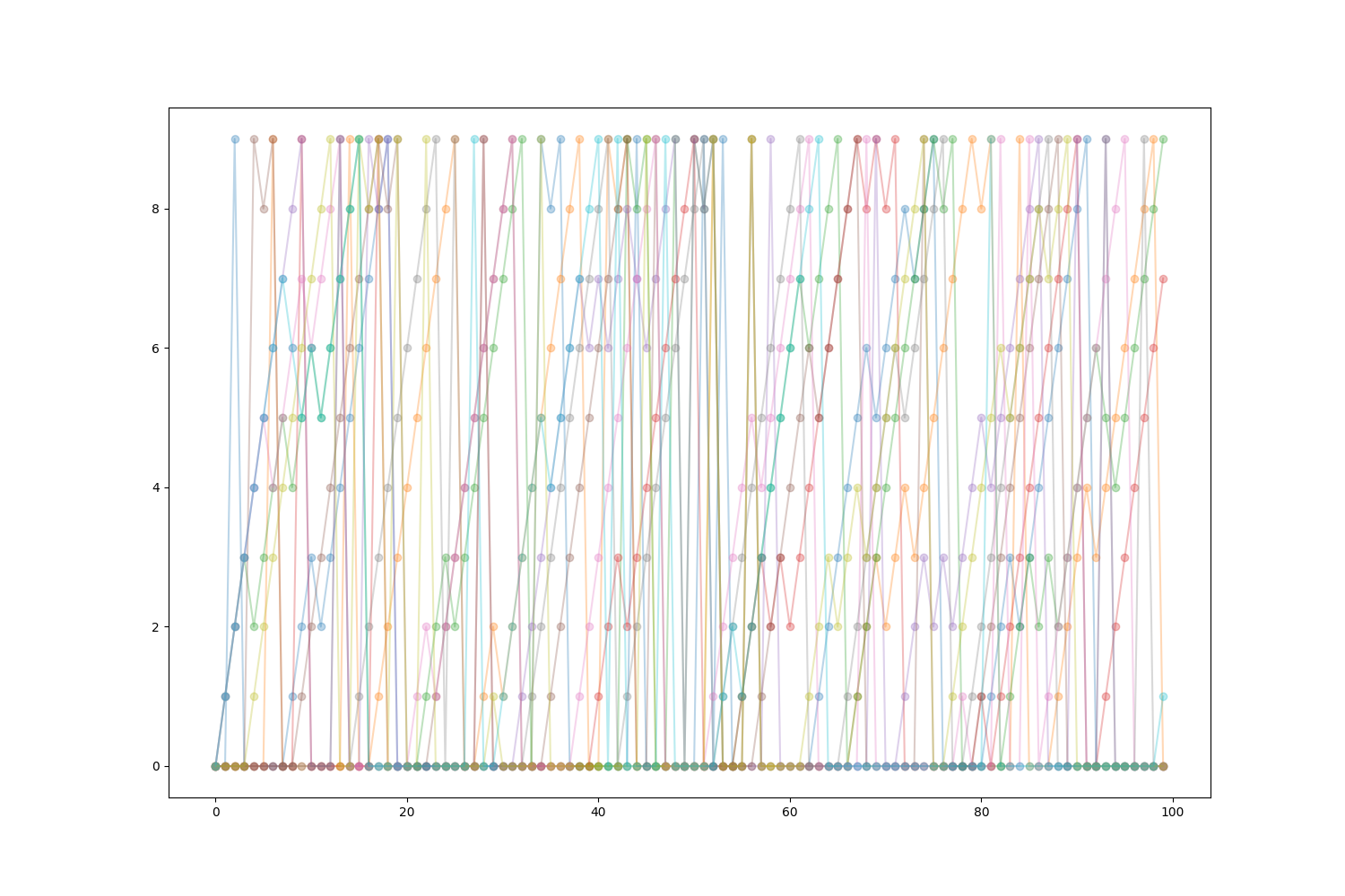
[<matplotlib.lines.Line2D object at 0x7f5969b62780>, <matplotlib.lines.Line2D object at 0x7f5969b63410>, <matplotlib.lines.Line2D object at 0x7f5969b624b0>, <matplotlib.lines.Line2D object at 0x7f5969b61be0>, <matplotlib.lines.Line2D object at 0x7f5969b607d0>, <matplotlib.lines.Line2D object at 0x7f5969b622a0>, <matplotlib.lines.Line2D object at 0x7f5969b60da0>, <matplotlib.lines.Line2D object at 0x7f5969b60ce0>, <matplotlib.lines.Line2D object at 0x7f5969b60e90>, <matplotlib.lines.Line2D object at 0x7f5969b61070>]

episodes = sample_episodes(n_episodes=100, length_episodes=100)
plt.hist((episodes[:, :50].flatten(), episodes[:, 50:].flatten()),
         density=True,
         label=["first 50 steps", "second 50 steps"])
plt.legend()


# Compute the closed-form solution for stationary distribution

<matplotlib.legend.Legend object at 0x7f59697a5670>

eigvals, eigvecs = np.linalg.eig(transition_matrix.T)
stationary = None
for idx in range(n_states):
    if np.isclose(eigvals[idx], 1):
        stationary = eigvecs[:, idx].real
        stationary /= stationary.sum()
print(f"Is stationary: {np.all(np.isclose(stationary @ transition_matrix, stationary))}")
print(stationary)


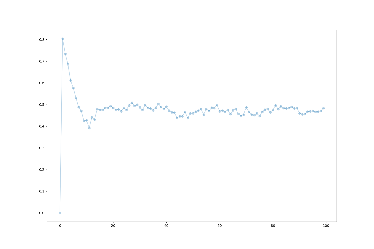
# ## Markov Reward Process

# Add a reward function and estimate the expected reward over time

Is stationary: True
[0.47368421 0.05263158 0.05263159 0.05263167 0.05263237 0.05263871
 0.05269575 0.05320915 0.05782976 0.0994152 ]

def reward_function(s):
    return int(s == 0)

def sample_episodes(n_episodes, length_episodes):
    episodes = np.zeros((n_episodes, length_episodes, 2), dtype=int)
    for idx_episodes in range(n_episodes):
        for idx_time in range(1, length_episodes):
            current_state = episodes[idx_episodes, idx_time - 1, 0]
            probs = transition_matrix[current_state]
            next_state = np.random.choice(n_states, p=probs)
            episodes[idx_episodes, idx_time, 0] = next_state
            episodes[idx_episodes, idx_time, 1] = reward_function(next_state)
    return episodes

episodes = sample_episodes(n_episodes=1000, length_episodes=100)
fig, ax = plt.subplots(1, 1, figsize=(15, 10))
ax.plot(np.arange(episodes.shape[1]), episodes[:, :, 1].mean(axis=0), '-o', alpha=0.3);


# Add a discount factor and estimate state values

[<matplotlib.lines.Line2D object at 0x7f59697069f0>]

def sample_episodes(n_episodes, length_episodes, start_state):
    episodes = np.zeros((n_episodes, length_episodes, 2), dtype=int)
    episodes[:, 0, 0] = start_state
    for idx_episodes in range(n_episodes):
        for idx_time in range(1, length_episodes):
            current_state = episodes[idx_episodes, idx_time - 1, 0]
            probs = transition_matrix[current_state]
            next_state = np.random.choice(n_states, p=probs)
            episodes[idx_episodes, idx_time, 0] = next_state
            episodes[idx_episodes, idx_time, 1] = reward_function(next_state)
    return episodes

def estimate_state_values(*, discount, start_state_list, **kwargs):
    state_values = {}
    for start_state in start_state_list:
        episodes = sample_episodes(start_state=start_state, **kwargs)
        discounted_rewards = episodes[:, :, 1] * np.power(discount, np.arange(episodes.shape[1]))
        returns = discounted_rewards.sum(axis=1)
        value = returns.mean()
        state_values[start_state] = value
        print(f"Value for state {start_state}: {value}")
    return state_values

state_values = estimate_state_values(discount=0.5,
                                     start_state_list=[n_states - 1, 0, 1],
                                     n_episodes=100,
                                     length_episodes=10)


# Compute the closed-form solution for the state values

Value for state 9: 0.82705078125
Value for state 0: 0.72212890625
Value for state 1: 0.0823828125

R = np.zeros(n_states)
R[0] = 1
np.linalg.solve(np.eye(n_states) - 0.5 * transition_matrix, 0.5 * transition_matrix @ R)


# ## MDP

# Add action to move up/down and update the transition matrix accordingly

array([0.74105284, 0.09069124, 0.00808578, 0.00789158, 0.01663844,
       0.03609746, 0.07836786, 0.17013997, 0.36938128, 0.80194284])

n_actions = 2  # up/down
idx = np.arange(n_states)
transition_matrix = np.zeros((n_states, n_states, n_actions))
transition_matrix[idx, (idx - 1) % n_states, 0] = 0.1
transition_matrix[idx, (idx + 1) % n_states, 0] = 0.9
transition_matrix[idx, (idx - 1) % n_states, 1] = 0.9
transition_matrix[idx, (idx + 1) % n_states, 1] = 0.1
print(f"normalised: {np.all(transition_matrix.sum(axis=1)==1)}")


# Adapt your sampling routine

normalised: True

def sample_episodes(n_episodes, length_episodes, start_state, policy):
    episodes = np.zeros((n_episodes, length_episodes, 3), dtype=int)
    episodes[:, 0, 0] = start_state
    for idx_episodes in range(n_episodes):
        for idx_time in range(1, length_episodes):
            current_state = episodes[idx_episodes, idx_time - 1, 0]
            action = np.random.choice(n_actions, p=policy[current_state])
            probs = transition_matrix[current_state, :, action]
            next_state = np.random.choice(n_states, p=probs)
            episodes[idx_episodes, idx_time, 0] = next_state
            episodes[idx_episodes, idx_time, 1] = reward_function(next_state)
            episodes[idx_episodes, idx_time, 2] = action
    return episodes


# Define a uniform policy and estimate state values

policy = np.zeros((n_states, n_actions))
policy[:, 0] = 0.5
policy[:, 1] = 0.5

estimate_state_values(discount=0.5,
                      start_state_list=[n_states - 1, 0, 1],
                      n_episodes=100,
                      length_episodes=10,
                      policy=policy);


# Change the policy to always go one step up and re-estimate the state values

Value for state 9: 0.30796875
Value for state 0: 0.153515625
Value for state 1: 0.3164453125

{9: np.float64(0.30796875), 0: np.float64(0.153515625), 1: np.float64(0.3164453125)}

policy = np.zeros((n_states, n_actions))
policy[:, 0] = 1
policy[:, 1] = 0

estimate_state_values(discount=0.5,
                      start_state_list=[n_states - 1, 0, 1],
                      n_episodes=100,
                      length_episodes=10,
                      policy=policy);


# Experiment with different policies and try to improve them

Value for state 9: 0.478203125
Value for state 0: 0.0597265625
Value for state 1: 0.0657421875

{9: np.float64(0.478203125), 0: np.float64(0.0597265625), 1: np.float64(0.0657421875)}

policy = np.zeros((n_states, n_actions))
policy[:int(n_states / 2), 0] = 0
policy[:int(n_states / 2), 1] = 1
policy[int(n_states / 2):, 0] = 1
policy[int(n_states / 2):, 1] = 0

estimate_state_values(discount=0.5,
                      start_state_list=[n_states - 1, 0, 1],
                      n_episodes=100,
                      length_episodes=10,
                      policy=policy);

Value for state 9: 0.60015625
Value for state 0: 0.299765625
Value for state 1: 0.587109375

{9: np.float64(0.60015625), 0: np.float64(0.299765625), 1: np.float64(0.587109375)}