Basic Example

This is a brief walk through some basic MusicFlower functionality.

Loading a File

We are using a MusicXML file as it is small enough to ship with the documentation. It can be loaded using the load_file() function

from musicflower.loader import load_file

# path to file
file_path = 'Prelude_No._1_BWV_846_in_C_Major.mxl'
# split piece into this many equal-sized time intervals
resolution = 50
# get pitch scape at specified resolution
scape = load_file(data=file_path, n=resolution)
print(scape.shape)

Out:

(1275, 12)

The result is an array with pitch-class distributions (PCDs), stored in a triangular map (see Triangular Maps). You can load multiple pieces using the load_corpus() function

from musicflower.loader import load_corpus
corpus, files = load_corpus(data=[file_path, file_path], n=resolution)
print(corpus.shape)

Out:

  0%|          | 0/2 [00:00<?, ?it/s]
 50%|#####     | 1/2 [00:00<00:00,  1.64it/s]
100%|##########| 2/2 [00:01<00:00,  1.69it/s]
100%|##########| 2/2 [00:01<00:00,  1.69it/s]
(2, 1275, 12)

The resulting array has the different pieces as its first dimension. Since we have loaded the same pices twice, we will transpose one version by a semitone to fake a different second piece

import numpy as np
corpus[1] = np.roll(corpus[1], shift=1, axis=-1)

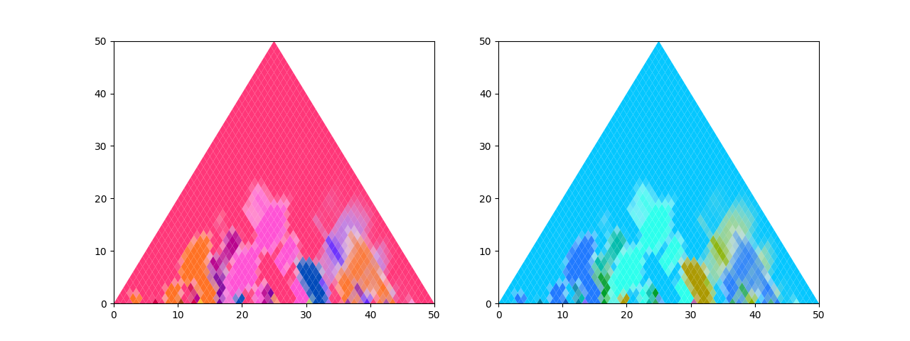
Key Scape Plots

Pitch scapes can be visualised in traditional key scape plots, which are the basis for the 3D visualisation provided by the MusicFlower package.

from musicflower.plotting import plot_key_scape
plot_key_scape(corpus)

More functionality, such as a legend for the used colours, is available via the PitchScapes library

import pitchscapes.plotting as pt
_ = pt.key_legend()

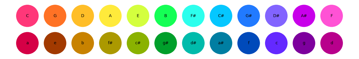
Colour

The key_colors() function can be used to get the corresponding triangular map of colours as RGB in [0, 1]. These are computed by matching each PCD against templates for the 12 major and 12 minor keys and then interpolating between the respective colours shown in the legend above.

from musicflower.plotting import key_colors
colors = key_colors(corpus)
print(colors.shape)

Out:

(2, 1275, 3)

Mapping to Fourier Space

The discrete Fourier transform of a PCD contains musically relevant information. In particular, the 5th coefficient is strongest for distributions that correspond to diatonic scales and can therefore be associated to the tonality of a piece: its amplitude indicates how “strongly tonal” the piece is (e.g. atonal/12-tone pieces have a low amplitude); its phase maps to the circle of fifths. The get_fourier_component() function provides amplitudes and phases of an array of PCDs

from musicflower.util import get_fourier_component
amplitude, phase = get_fourier_component(pcds=corpus, fourier_component=5)

Mapping to 3D Space

The amplitude and phase of the Fourier component provide polar coordinates for each of the PCDs. (The phase also strongly correlates with the colours, even though they were computed using template matching, not Fourier components.) In the key scape plot above, we have two other dimensions for each PCD: time on the horizontal axis and the duration on the vertical axis (i.e. center and width of the respective section of the piece). Together, this can be used to map each PCD to a point in 3D space as follows.

We use spherical or cylindrical coordinates with the phase as the azimuthal/horizontal angle, the duration for the radial component, and the amplitude for the vertical component/angle (cylinder/sphere). This is done by the remap_to_xyz() function, which also provides some additional tweaks (see its documentation for details). Note that time is not explicitly represented anymore, but can be included through interactive animations (see below).

from musicflower.util import remap_to_xyz
x, y, z = remap_to_xyz(amplitude=amplitude, phase=phase)

3D Plot

This can be visualised in a 3D plot as follows

from musicflower.plotting import plot_all
plot_all(x=x, y=y, z=z, colors=colors)

Time as Animation

We can add the time dimension using an interactive slider and/or animation. The slider represents time in a normalised [0, 1] interval over the piece duration. When moving the slider, a line is drawn from the top, through the triangular map to the point at the bottom corresponding to the current slider position. In the normal key scape plot from above, this would simply be a straight line from the top down to the bottom; in the 3D plot it winds through tonal space (also see Time Traces).

plot_all(x=x, y=y, z=z, colors=colors, do_plot_time_traces=True)